

This is not a call for data engineers to become mathematicians. This is a call to add back the formality that “engineering” requires. No one considers a bridge safe because it hasn’t fallen down yet. But this is more or less the standard that data pipelines and machine learning models are held to.
This article is the third and last part of a series on building data systems that prevent errors by design. Part 1 argued that data systems are in an urgent need of a discipline that prevents errors by design. Part 2 turned those steps of proving, checking and monitoring into a practical recipe, with a worked example.
This part will use the same example pipeline but will focus on the “proving” step. We will go through different levels of arguing about the systems we build, from least to most complex. And how to decide which level of argument a property deserves.
We saw how writing a simple argument can rule out errors earlier. This is the good news. In my experience, the less formal levels catch most of the errors. The more formal end of the spectrum is mainly for the few properties that are both expensive to get wrong, and easy to get wrong.
This is part one of the Towards a Data Discipline series:
The first post explained the main principles.
The second gives a step by step recipe to follow.
And this last part focuses on one specific step: formal arguments to prove what we are building is correct.
Let’s agree on what we mean by “prove”
Recall the definition from Part 1 of this series: Given a function f over inputs I, a precondition P and a postcondition Q, a proof establishes that ∀ x ∈ I : P(x) ⇒ Q(x, f(x)).
In other words, that for every input: if this input satisfies the preconditions, the postcondition is satisfied for the input/output pair.
So a proof does not guarantee that the system will not fail. It relies on the precondition P, and it relies on how we model the system. Inputs in real life can violate P, and code can drift from the initial design. This is why we still use checking and monitoring. But a proof also forces us to reason about our design, which helps us define which assumptions we rely on and what errors we may run into and makes the checking and monitoring steps easier.
In the rest of this article I will actually use the word “Argument” more. This is because not all arguments are proofs in the strict sense, and when I said “prove what you can” what I really meant is to argue for these properties.
The worked example
We will use the same worked example from Part 2.
As a reminder, we have a service that emits two kinds of events: orders or refunds
Each has: id, an amount in euros and the time it happened. Events are delivered at least once, so duplicates can happen, and they can arrive late.
We must produce a table to show to the finance team, daily_revenue, with one row per day containing: gross sales, refunds.
In our design we decided that: Every morning at 06:00 UTC, the run for day D (on D+1) recomputes the partitions for D-3 to D.
The assumptions we made along the way:
- A1. Events arrive within 24h.
- A2. Every event has a unique id (a duplicate is identical to the original).
- A3. Amounts are positive, in euros, in whole cents.
- A4. A “day” is a calendar day in UTC.
How hard should we prove it
As we mentioned in Part 2, we asked two questions about the properties we want to prove:
What does it cost us if this property is false?
How easy is it to get the argument wrong?
As we did in our example, the properties end up with a proof chosen from one of the following types:
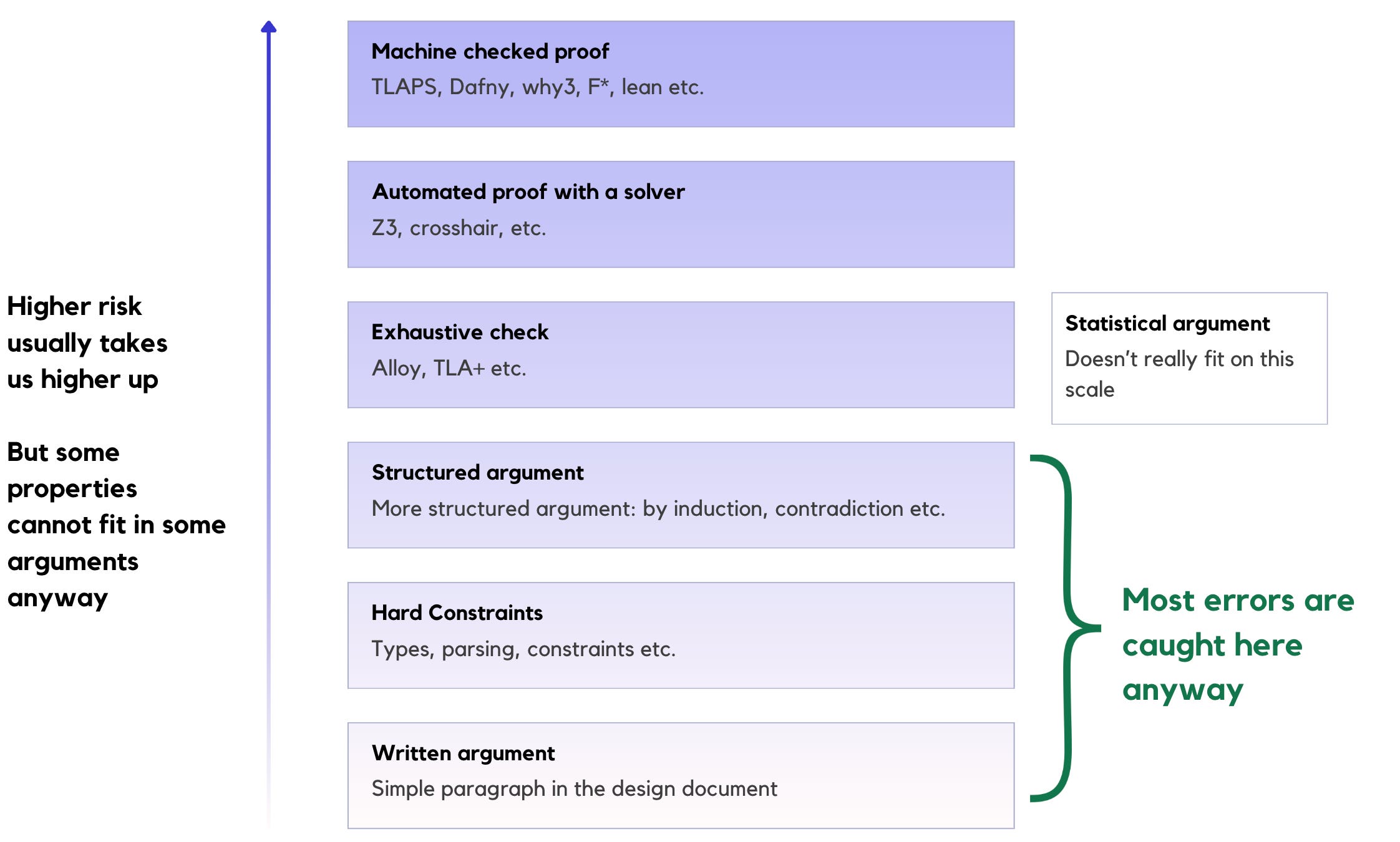
Here is an example of ways to prove that go from easier to write to harder to write (which doesn’t mean better):
A written argument: written in the design document or another type of text, a reviewer can spot wrong beliefs and reasoning errors. It doesn’t guarantee there are no mistakes.
Hard constraints (Construction and types): simply making the invalid states impossible to represent, so that nothing is left to prove (for example, a string variable that contains ‘true’ or ‘false’ is obviously better off being a boolean). This includes database constraints, parsing, validated types. In machine learning: monotonic constraints, domain-constrained outputs, equivariant architectures and other types of constraints can be added depending on the use case.
A structured argument: this is a step up from the written argument. The proof techniques you may have learned and stopped using (induction over days/partitions, contradiction, contraposition etc.). This is still written text, reviewed by people, but the structure makes it less likely to fail. It requires a bit more time than a written argument.
Exhaustive checking: there are tools that help you write a small model of the design and let a tool explore every state (up to a bound). Alloy for relations/data models, TLA+ for concurrency and orchestration, P for distributed state machines. There are tools for the code itself, I personally have never used any of these but there are bounded model checkers such as CBMC for C and Kani for Rust. The reason for this type of checking, as Daniel Jackson puts it, is that most design issues show up in small examples (exploring all of them is worth more than sampling large ones).
Automated proof with a solver: these are only possible in specific cases, you basically state the claim as logical formulas and let an SMT solver, such as Z3, prove it for every input or give a counterexample. You can call Z3 from Python in a dozen lines, as we will. For Python functions, we have CrossHair checking contracts. For SQL, some promising tools exist such as SQLSolver and VeriEQL but they are not yet everyday tools (solvers struggle with non-linear arithmetic and complex data structures, so this level is more for small but critical claims).
Machine-checked deductive proof: in these types of proofs you write the code together with its specification and prove that they match. Tools include: Dafny (can compile verified code to Python, and other languages), Why3, F*. Proof assistants such as Lean, Rocq and Isabelle. TLA+ has TLAPS. This is a very strong guarantee, but it also implies the highest cost in time and expertise.
“Statistical” arguments: this is not a proof and doesn’t really fit in this list. But some properties cannot be proven that way: how long a job takes to run, how quickly an API, how accurate a model is etc. For these cases, we can still make a good case using statistics (Evaluating a model on a separate validation set is an example). Kochenderfer’s group is one of those who have thought deeply about such arguments and how they apply for airplane collision avoidance as an example. They usually name three types of tasks: falsification (finding any input that causes failure), most-likely failure (finding errors that are more probable), and failure probability estimation (finding out how often something fails). The book Algorithms for Validation includes these along with formal methods and monitoring (and is part of the inspiration to this series as well).
Now let’s see where the properties we deduced in Part 2 fit here. We already argued for P1 and P2, so we will only focus on the rest. Here is the register with the type of proof we select in bold.
Proof register:
P3. daily revenue matches the finance team definition. Type guarantees and a written argument. Depends on A2, A3 and A4.
P4. daily revenue is the same whether the table was built daily or rebuilt once (incremental equals full): a structured argument, by induction. Depends on P1, P6 and P7.
P5. the job is ready by 07:00: statistical argument by running multiple times (on the edge examples) and reporting the distribution of time it takes to run.
P6. no on-time event is missed: if an event satisfies A1, it is accepted before the last run that recomputes the day of that event. Machine-checked, with SMT solver. Depends on A1 and on the scheduler.
P7. isolation: an overlapping retry never overwrites newer results. Validated through an exhaustive check of possible interleavings.
This is just a way of seeing these properties and where each type of argument may be more appropriate. In our example, we already went through P1-P2 through a simple written argument. This post will focus on the remaining properties and how we can argue for them.
How to argue for a property
Hard constraints: make illegal states impossible
If an invalid state cannot be represented, it cannot be reached. For example, a string column holding “true” and “false” is better off being a boolean.
This level of argument should be used very often (and is used very often) in databases through constraints and type definitions. It also exists in machine learning in the form of monotonic constraints, outputs restricted to a valid domain, equivariant architectures etc.. A pricing model trained with a monotonic constraint on a variable does not need a proof that this variable will follow that rule. In training sets as well, point-in-time joins can be used to avoid leakage.
Now let’s look at our example P3. daily revenue matches the finance team definition. In the pseudocode below, the Event type can’t hold a negative amount, a naive timestamp or an event later than we allow, so nothing downstream needs to consider one (there are better types to write this code, but this is enough to show our point)
# imports and definitions constants here...
class ContractViolation(ValueError):
    """The record goes to quarantine, after this violation"""

@dataclass(frozen=True)
class Event:
    event_id: str
    kind: Literal["order", "refund"] # "order" or "refund"
    amount: Decimal # euros, whole cents, > 0 (A3)
    occurred_at: datetime  # timezone-aware
    received_at: datetime  # timezone-aware

    def __post_init__(self):
        if self.kind not in ("order", "refund"):
            raise ContractViolation(f"unknown kind: {self.kind!r}")
        if self.amount <= 0 or self.amount != self.amount.quantize(CENT):
            raise ContractViolation(f"not a positive whole-cent amount: {self.amount}")
        ...
        if self.received_at - self.occurred_at > MAX_DELAY:
            raise ContractViolation("arrived later than A1 allows")

    @property
    def day(self) -> date:  # A4: a calendar day in UTC
        return self.occurred_at.astimezone(timezone.utc).date()

def parse_event(raw: dict) -> Event:
    """Once we parse here, the assumptions will hold for the rest of the code"""
    return Event(
        event_id=str(raw["id"]),
        kind=raw["kind"],
        amount=Decimal(str(raw["amount"])),
        occurred_at=datetime.fromisoformat(raw["occurred_at"]),
        received_at=datetime.fromisoformat(raw["received_at"]),
    )
A type checker will reject code that tries to build an Event that doesn’t follow our assumptions. I talked about parsing as a “check” in part 2, and now I mentioned it as an argument. Well, it is both, it’s a check at runtime, but writing this earlier is a proof for what happens downstream. Now that we have this type guarantee, we can continue with the written argument.
Whichever the use case, this type of argument is a strong and cheap guarantee so check for what types of constraints are needed to guarantee your specific properties.
Structured arguments
Now let’s look at a more structured type of proof.
At the end of the day, this is still reviewed by people. But with a structure that makes it easy to spot any steps we skip, or any mistakes we make while thinking. This is where we can use arguments such as: induction, contradiction, contraposition, etc.
Here’s an example for our case: P4. incremental equals full: this property depends on a precondition: every event arrives in time for one of the runs that recompute the day of the event (either the run on the same day or in 3 days after). That precondition is P6, and we will prove P6 later so for now let’s assume it holds. It also depends on P7 because it assumes runs happen one after the other.
Proof by induction
Claim: after the run for day D, the result of every partition up to D equals the result of a full rebuild from all accepted events.
Base case: before the first run, the table is empty and there is nothing to compare.
Inductive step:
Assume the claim holds after the run for day D.
Let us consider accepted events between the run for day D and the next on D+1.
- These events belong either to a day from D-2 to D+1, or to a later day, not yet published.
- The run for D+1 recomputes exactly partitions from D-2 to D+1, each of them equals the full rebuild (by P1).
- Partitions older than D−2 are not touched by this run. By P6, none of the newly accepted events belongs to them. So they are unchanged, and by the induction hypothesis they equal the full rebuild.
So the claim holds after running D+1
Notice how this made use of: P1 and P6, while assuming P7. Trying to prove properties usually brings up what you depend on, and how confident you are in those dependencies.
Exhaustive Check
Testing tries a few cases, but an exhaustive checker tries all of them, up to a certain bound. You write a model of your design, and let a tool explore every state that can be reached. Alloy is such a tool for data models and relations. TLA+ works best for concurrency and orchestration. These tools will catch if something can go wrong within the bounds.
A small model is usually enough here, because most design errors are small. Daniel Jackson has called this the small scope hypothesis: if a design is flawed, a few small examples usually expose the flaw. This is also why testing as a first pass is encouraged, despite what I said earlier about testing. A test that finds an error early is good as long as it doesn’t make us overconfident.
The obvious, and heavily cited, example is that of AWS engineers who had reported that TLA+ caught design errors in their systems that they would not have found otherwise. And engineers became productive with TLA+ in two to three weeks (which is a small price to pay for a critical system, it seems that they have moved on from this recently, and use P language instead to model systems and PObserve to check the logs are following the model).
For our pipeline example, this type of argument would be overkill. But imagine a scenario where a job fails on day D, we keep retrying until D+1, while the job for D+1 itself already started. Two jobs are now writing the same three days at the same time. Which values end up in the table? Does idempotence still hold? Problems like this are what people tend to reason about worse. If you have taken a parallel programming course you may be better trained to reason in such a way. But even then, when the systems are complex enough, and critical enough, using exhaustive checks can let the machine examine what your mind is too small to hold.
So let us check it anyway for the sake of example:
P7. isolation: an overlapping retry never overwrites newer results
Once again, this exhaustive check will only check for the model we defined in this code. Our actual code can still be different or drift away from this model, what we basically do here is we take our data pipeline design → simplify into a model → enumerate and check interleavings.
Runs can overlap, but neither run can execute its own steps out of order.
We will add an input variable calledfencing, when it is true older runs are not allowed to overwrite newer runs. We will see here that when this is set to false we end up with a lot of possibilities of interleavings (in our case, more than half of the time)from itertools import combinations def run(name, partitions): """This models the run as a sequence of steps, starting with 'start' followed by the partitions""" return [(name, "start")] + [(name, p) for p in partitions] def interleavings(a, b): """Every order in which the steps of two runs can happen.""" n = len(a) + len(b) for positions in combinations(range(n), len(a)): ia, ib = iter(a), iter(b) yield [next(ia) if i in positions else next(ib) for i in range(n)] def execute(steps, fenced): """Executes the given steps with optional fencing. Fencing means that a partition will not be updated with an older snapshot.""" clock, snapshot, table = 0, {}, {} for name, step in steps: # The "start" step records when the run begins # Each number represents a partition it writes if step == "start": clock += 1 snapshot[name] = clock elif fenced and table.get(step, 0) > snapshot[name]: continue # here we do not overwrite a partition with older data else: # here we update the partition with the current snapshot of the run table[step] = snapshot[name] return table, snapshot fenced = False D=10 retry = run("retry of day D", range(D - 3, D + 1)) nxt = run("run for D+1", range(D - 2, D + 2)) total = bad = 0 for steps in interleavings(retry, nxt): table, snapshot = execute(steps, fenced) # each partition must end up with the newest snapshot that wrote it expected = {} for name, partitions in (("retry of D", retry), ("run for D+1", nxt)): for _, p in partitions[1:]: expected[p] = max(expected.get(p, 0), snapshot[name]) total += 1 bad += table != expected print(bad, total) # (143, 252) # if you set fenced = True, we get no issues
What we have shown here is that “assuming this model holds, and fencing is enabled, we prevent older runs from overwriting newer data in all possible interleavings” This doesn’t show our pipelines truly follows this model, nor that fencing is enabled. And that if fencing is not enabled, this can definitely happen.
We can make this safe in practice for example by forcing the orchestrator to never run two of these jobs at once, or to have a version of the snapshot within the run.
Automated proof with a solver
Now let’s look at P6 which we promised to use an SMT solver for: P6. no on-time event is missed.
If an event satisfies the assumption (A1, arrives within 24h) the event is received before the last run that recomputes its day.
What a solver does: an SMT solver, such as Z3, takes a set of conditions on some unknowns, for example x > 3 and x + y = 10. It then does one of two things.
- Finds values that satisfy every condition at once
- Or it proves that no such values exist.
It does not try values one by one. It reasons about the conditions in a similar way that you would solve an equation instead of trying all numbers that may or may not solve it.
How that becomes a proof: in our case, we ask the solver to find a counterexample that satisfies A1 and is still missed. If it finds one, then we have an error. If it reports that no such event can exist, then P6 holds as long as the preconditions are valid.
A written argument for this simple case could be short and convincing enough. But a solver should be considered if we have the time to invest, and consider this property critical enough. Here’s an example using Z3
from z3 import Ints, Solver, sat, unsat
from revenue import DAYS_BACK, MAX_DELAY, RUN_START

DAY = 86_400 # in seconds

def seconds(t):
    return int(t.total_seconds())

def find_missed_event(days_back=DAYS_BACK, run_start=RUN_START, max_delay=MAX_DELAY):
    """Find event that:
      - satisfies A1
      - and is still missed.
      Missed here means: it is received only at or after the start of the
      last run that can recompute it"""
    occurred, received = Ints("occurred received")  # defined in seconds since 1970, UTC
    day = occurred / DAY # integer division: its UTC day (A4)
    # The run for day D starts on D+1 and recomputes D-days_back up to D,
    # so day d is last recomputed by the run for d + days_back.
    last_run = (day + days_back + 1) * DAY + seconds(run_start)
    solver = Solver()
    solver.add(occurred >= 0,
               received >= occurred,
               received - occurred <= seconds(max_delay),  # A1
               received >= last_run)                       # ...and yet missed
    result = solver.check()
    if result == unsat:
        return None # proved: no such event exists
    if result == sat:
        return solver.model() # a counterexample
    raise RuntimeError("The solver was unable to decide.")
In simple words, the function states three facts: when the event occurred, when it was received, and that the delay between the two respects A1. Then it adds the condition that the event arrived too late. If find_missed_event() returns None, no event can satisfy this. This also makes things more robust to changes in the code, if someone changes the DAYS_BACK in the code, this property will be validated again.
A little word of honesty: as you see in the end, a solver can answer sat, unsat or unknow. When I first wrote this, it worked such that unknown was also considered a proof. Errors like this can happen especially for someone like myself who is very new to z3 (I’m sure experienced people would have spotted this faster). But this is just a word of caution again, that the guarantees of these arguments are great, but they are not completely free of flaws.
You can also test the SMT solver by going into a case where you know it should fail (setting days back to 0 in our example) and see that it comes up with counterexamples.
The solver obviously proves this for a model of the design, not for what happens when we hand it over to the orchestrator.
Statistical arguments
I left P5 last as it is a different kind of argument. P5. ready by 07:00: assuming the run starts at 6:00 it must finish within the hour. A proof cannot really establish this. But we can use a statistical argument.
P5. ready by 07:00 : Before we start this argument let’s make an assumption, we can add this to our assumptions register and check for it when monitoring: A5. daily volume never exceeds twice the volume of the busiest day observed so far.
Let’s say we now run twice the maximum volume observed 300 times on our cluster. And say the slowest run takes 19 minutes. It feels like we have enough evidence, but the evidence is weaker than it feels. 300 runs without a single overrun allow us to say, with 95% confidence, that a run overruns less than one time in a hundred. But we don’t know the tail of our model.
Here are four directions we could go:
Accept the risk: and consider this to be enough for our case. After all, the finance team wants to guarantee this just 90% of the time.
Run it more: 3000 clean runs would bring those down to one in a thousand. But this is 10x more expensive.
Make an assumption about the tail distribution: and add we add that distribution as an assumption to the register. We can use it to estimate how likely a run is to go beyond an hour. But because the distribution is an assumption we may want to verify it and monitor for it depending on how critical it is.
Sample the harder cases: if we are interested in the rare event, this problem is what failure probability estimation deals with. Simulating ordinary days over and over is not an efficient way to learn about the rare events. One of the methods that can be used here is importance sampling, one of the families of methods Kochenderfer et al. survey in Algorithms for Validation. This means sampling from a distribution biased towards errors (more volume, more late events etc.). We can then give each run a weight: how likely the conditions are on an ordinary day, divided by how likely we made them be in our sampling distribution. The weights correct for the bias we introduced, so the estimate still describes ordinary days, but now most of your runs are spent where the errors are most likely. However, this requires a distribution of what a “normal” day looks like. We usually don’t have this, which means that if we take this route we need to model this distribution and add that as a new assumption, by fitting it to history and then monitoring like any other assumption. Once again, Algorithms for Validation is the place to read about such strategies.
Whichever way we go, what they all should have in common is a form of transparency: stating the confidence, and writing down the assumptions we are making so that we can monitor them later.
But the code will drift away
If you prove for your current design, the code can (will) drift away with time. So how can we keep it consistent with our proofs?
Testing can close some of the gap. For example, property-based testing states the property’s own claim, and can look for inputs that break it. This is what Hypothesis is for in Python as an example. This test is still only sampling, but it samples whether the code stays faithful to our argument.
from hypothesis import given, settings, strategies as st

# events(): a strategy for well-formed, on-time events (A1 to A3), duplicates included
@given(st.lists(events(), max_size=50))
@settings(max_examples=500)
def test_incremental_equals_full(evts):
    # replay_daily_runs: run the job every morning, on what had arrived by then
    # rebuild_from_scratch: one run at the end, over everything accepted
    assert replay_daily_runs(evts) == rebuild_from_scratch(evts)
On our design, this would pass 500 generated histories in about two seconds. We are still just sampling but we are checking if the code still behaves in a way that the proof expects.
It’s always good practice to make sure the test can fail. Try an example where it should fail and Hypothesis should find a counterexample in a few seconds.
And of course, this is not a guarantee that the code will not drift. There are other tools that can improve this. CrossHair for example can explore Python code symbolically, using Z3 in the background. At the far end of the arguments Dafny closes it entirely (the code and the proof are tied together and the program wouldn’t compile unless the proof holds). But let’s be honest, most data teams will not go that far. But in case of very critical systems, we have to know what exists and what tradeoffs we are making.
Conclusion
Most of the guarantees of correctness in this series came from the simple parts: a falsifiable statement, an assumptions register, a few written arguments, type constraints, and parsing. The expensive tools (solvers, model checkers, proof assistants) only become interesting on one or two properties at most (which we may have exaggerated in this example).
And if you use language models for assistance writing code (who doesn’t at this point), just make sure you do the reasoning yourself first. Language models can assist you in reviewing it, they can assist in spotting flaws, as well as assist in writing and reviewing Z3 or Hypothesis code or similar. But if we completely rely on them, we not only risk having them solve something different from what we define as correct. I’m writing a few skills that can help in this process that I will share both here and by email as soon as they’re ready.
This whole series can be put in three lines:
Prove what you can, so that some errors are impossible by construction.
Check at the boundaries, so that the preconditions of the proofs also hold.
Monitor the rest, and give every alert an owner and a checklist.
None of this is new. What I hope this series adds is a practical way to apply it to data systems, without turning every engineer into a mathematician. If you build data or ML systems, I would genuinely like to hear if this is helpful at all.